import pandas as pd
import numpy as np
import sklearn.linear_model
import matplotlib.pyplot as plt
import sklearn.preprocessing
import sklearn.impute
import seaborn as sns
import sklearn.tree선형모형의 적
linear_model
preprocessing
impute
tree
우리의 주적은 북한인데, 선형모형의 적은?
해당 자료는 전북대학교 통계학과 최규빈 교수님의 강의 내용을 토대로 재구성되었음을 밝힙니다.
1. 라이브러리 imports
2. 선형모형의 적
A. 결측치의 존재
문제 : 데이터에서 누락된 값이 있는 경우, 선형모델이 돌아가지 않는다.
- 해결방안
1 : 결측치를 제거
결측치가 포함된 열을 제거
결측치가 포함된 행을 제거
둘을 혼합
- 결측치를 impute
train에서는 fit_transform, test에서는 transform
train, test에서 모두 fit_transform
임의의 값으로 일괄 impute
interploation(이미지 또는 시계열, 근처의 값과 자연스럽게 연동되도록 만들 수 있음)
~train, test data를 합쳐서 fit_transform~ 이건 정보누수로 실격사유가 된다
- 사용 가능한 코드나 모듈
isna(),dropna(),sklearn.inpute의 하위 모듈 등.
### B. 다중공선성의 존재
문제 : 데이터의 설명변수가 역할이 겹칠 경우, 선형모형의 일반화 성능이 좋지 않음.
- 해결방안
변수 제거 > 설명변수 간 corr을 파악하고, 느낌적으로 제거 > > PCA 등 차원축소기법을 이용한 제거
공선성을 가지는 변수를 모아 새로운 변수로 변환 > 느낌적으로 변환 > > PCA를 이용한 변환
Lasso, Ridge 등 패널티 계열을 사용 > Lasso : l1 / liblinear > > Ridge : l2 > > Elastic net
- corr파악 후 느낌적으로 제거의 예시
df = pd.read_csv("https://raw.githubusercontent.com/guebin/MP2023/main/posts/employment_multicollinearity.csv")
X = df.loc[:,'gpa':'toeic2']
X| gpa | toeic | toeic0 | toeic1 | toeic2 | |
|---|---|---|---|---|---|
| 0 | 0.051535 | 135 | 129.566309 | 133.078481 | 121.678398 |
| 1 | 0.355496 | 935 | 940.563187 | 935.723570 | 939.190519 |
| 2 | 2.228435 | 485 | 493.671390 | 493.909118 | 475.500970 |
| 3 | 1.179701 | 65 | 62.272565 | 55.957257 | 68.521468 |
| 4 | 3.962356 | 445 | 449.280637 | 438.895582 | 433.598274 |
| ... | ... | ... | ... | ... | ... |
| 495 | 4.288465 | 280 | 276.680902 | 274.502675 | 277.868536 |
| 496 | 2.601212 | 310 | 296.940263 | 301.545000 | 306.725610 |
| 497 | 0.042323 | 225 | 206.793217 | 228.335345 | 222.115146 |
| 498 | 1.041416 | 320 | 327.461442 | 323.019899 | 329.589337 |
| 499 | 3.626883 | 375 | 370.966595 | 364.668477 | 371.853566 |
500 rows × 5 columns
X.corr()| gpa | toeic | toeic0 | toeic1 | toeic2 | |
|---|---|---|---|---|---|
| gpa | 1.000000 | -0.033983 | -0.035722 | -0.037734 | -0.034828 |
| toeic | -0.033983 | 1.000000 | 0.999435 | 0.999322 | 0.999341 |
| toeic0 | -0.035722 | 0.999435 | 1.000000 | 0.998746 | 0.998828 |
| toeic1 | -0.037734 | 0.999322 | 0.998746 | 1.000000 | 0.998721 |
| toeic2 | -0.034828 | 0.999341 | 0.998828 | 0.998721 | 1.000000 |
pandas의 데이터프레임에는 자체적으로 해당 메소드를 지원한다.
sns.heatmap(X.corr(), annot = True)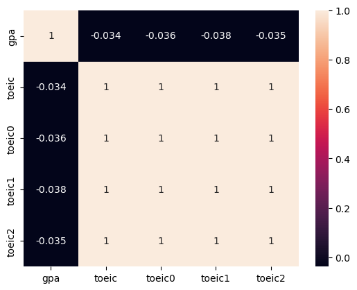
- toeic과 유사 toeic끼리 상관성이 짙네?
제거한다.
C. 관련이 없는 변수의 존재
문제 : 데이터에서 불필요한 설명변수가 너무 많을 경우, 선형모형의 일반화 성능이 좋지 않음.(overfitting)
예시 : 고객이름, ID, Index 관련 변수(물론 얘네들도 어딘가 쓸모가 있을 수도 있다…)
- 해결방법
변수 제거 > (y, X)의 corr을 파악하고 느낌적으로 제거(위에서와 달리 관련이 있어야 한다.) > > PCA를 이용한 제거 > > Lasso를 이용한 제거(여기서 Ridge는 사용하면 안된다. 해당 모듈은 유사한 것들의 계수 합이 일정하도록 조정하는 거니까…)
더 많은 데이터를 확보 > 하지만 이는 어렵다… 어떤 변수가 관련이 없다는 것을 파악하기 위해선 데이터를 많이 가져와야 하는데, Feature의 수가 많아질 때 필요한 데이터의 수는 지수적으로 증가한다.
- 느낌적으로 제거 예시
df_train.corr()| toeic | gpa | employment | balance0 | balance1 | balance2 | |
|---|---|---|---|---|---|---|
| toeic | 1.000000 | -0.033983 | 0.260183 | 0.002682 | 0.110530 | 0.024664 |
| gpa | -0.033983 | 1.000000 | 0.711022 | -0.025197 | 0.005272 | 0.020794 |
| employment | 0.260183 | 0.711022 | 1.000000 | -0.007348 | 0.036706 | 0.032284 |
| balance0 | 0.002682 | -0.025197 | -0.007348 | 1.000000 | -0.059167 | 0.040035 |
| balance1 | 0.110530 | 0.005272 | 0.036706 | -0.059167 | 1.000000 | -0.030215 |
| balance2 | 0.024664 | 0.020794 | 0.032284 | 0.040035 | -0.030215 | 1.000000 |
sns.heatmap(df_train.corr(), annot = True)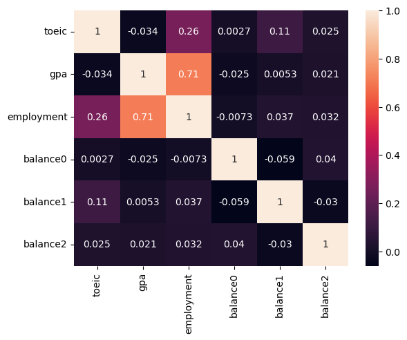
balance0 ~ 2는employment와의 상관성이 낮다. 따라서 제거하고 분석한다.
## 1
X = df_train.loc[:, :'gpa']
y = df_train.employment

## 2
predictr = sklearn.linear_model.LogisticRegression()

## 3
predictr.fit(X, y)

## 4
predictr.score(X, y)0.882- Lasso를 이용한 제거 예시
np.random.seed(1)
df = pd.read_csv('https://raw.githubusercontent.com/guebin/MP2023/main/posts/employment.csv')
df_balance = pd.DataFrame((np.random.randn(500,3)).reshape(500,3)*1,columns = ['balance'+str(i) for i in range(3)])
df_train = pd.concat([df,df_balance],axis=1)
df_train| toeic | gpa | employment | balance0 | balance1 | balance2 | |
|---|---|---|---|---|---|---|
| 0 | 135 | 0.051535 | 0 | 1.624345 | -0.611756 | -0.528172 |
| 1 | 935 | 0.355496 | 0 | -1.072969 | 0.865408 | -2.301539 |
| 2 | 485 | 2.228435 | 0 | 1.744812 | -0.761207 | 0.319039 |
| 3 | 65 | 1.179701 | 0 | -0.249370 | 1.462108 | -2.060141 |
| 4 | 445 | 3.962356 | 1 | -0.322417 | -0.384054 | 1.133769 |
| ... | ... | ... | ... | ... | ... | ... |
| 495 | 280 | 4.288465 | 1 | -1.326490 | 0.308204 | 1.115489 |
| 496 | 310 | 2.601212 | 1 | 1.008196 | -3.016032 | -1.619646 |
| 497 | 225 | 0.042323 | 0 | 2.005141 | -0.187626 | -0.148941 |
| 498 | 320 | 1.041416 | 0 | 1.165335 | 0.196645 | -0.632590 |
| 499 | 375 | 3.626883 | 1 | -0.209847 | 1.897161 | -1.381391 |
500 rows × 6 columns
로지스틱 선형 회귀가 필요한 경우이다. 로지스틱 또한 penalty 계열 분석을 할 수 있다.
## 1
X = df_train.drop('employment', axis = 1)
y = df_train.employment

## 2
predictr = sklearn.linear_model.LogisticRegressionCV(Cs = [0.1, 1, 10, 100], penalty = 'l1', solver = 'liblinear', random_state = 42)

## 3
predictr.fit(X, y)

## 4
predictr.score(X, y)0.876predictr.coef_array([[0.00260249, 1.41401358, 0. , 0. , 0. ]])s = pd.Series(predictr.coef_.reshape(-1)) ## 시리즈의 경우 1차원의 입력값만 받는다.
s.index = X.columns
stoeic 0.002602
gpa 1.414014
balance0 0.000000
balance1 0.000000
balance2 0.000000
dtype: float64위에서 쓸모없는 것을 제거하고 분석한 것에 비해 점수가 낮지만, 쓸모없는 것이라는 사실을 모르는 상황에서는 Lasso가 상당히 괜찮다.
### D. 이상치의 존재
문제 : 이상치가 존재할 경우 전체 모형이 무너질 수 있음
- 해결방법
이상치를 제거하고 분석 > 느낌적으로 제거 > > 이상치를 감지하는 지표를 사용하여 제거 > > 이상치를 자동으로 감지하는 모형 사용하여 이상치 제거 후 분석
로버스트 선형회귀 계열을 이용 > 이상치에 큰 영향을 받지 않음 >
sklearn.linear_model.HuberRegressor등이상치를 완화시키는 변환을 사용 >
sklearn.preprocessing.PowerTransformer를 이용
np.random.seed(43052)
temp = pd.read_csv('https://raw.githubusercontent.com/guebin/DV2022/master/posts/temp.csv').iloc[:100,3].to_numpy()
temp.sort()
ice_sales = 10 + temp * 0.5 + np.random.randn(100)
ice_sales[0] = 50
df_train = pd.DataFrame({'temp':temp,'ice_sales':ice_sales})[:10]
df_train| temp | ice_sales | |
|---|---|---|
| 0 | -4.1 | 50.000000 |
| 1 | -3.7 | 9.234175 |
| 2 | -3.0 | 9.642778 |
| 3 | -1.3 | 9.657894 |
| 4 | -0.5 | 9.987787 |
| 5 | -0.3 | 10.205951 |
| 6 | 0.3 | 8.486925 |
| 7 | 0.4 | 8.817227 |
| 8 | 0.4 | 8.273155 |
| 9 | 0.7 | 8.863784 |
transformr = sklearn.preprocessing.PowerTransformer()

transformr.fit_transform(df_train)
array([[-1.40729341, 2.42405408],
[-1.31406689, -0.18677452],
[-1.13030154, 0.16485704],
[-0.50278108, 0.17667635],
[-0.02130412, 0.41617603],
[ 0.13926015, 0.55696978],
[ 0.81742569, -1.03040835],
[ 0.96759638, -0.62032873],
[ 0.96759638, -1.33362249],
[ 1.48386844, -0.56759919]])x, y = transformr.fit_transform(df_train).T
x, y(array([-1.40729341, -1.31406689, -1.13030154, -0.50278108, -0.02130412,
0.13926015, 0.81742569, 0.96759638, 0.96759638, 1.48386844]),
array([ 2.42405408, -0.18677452, 0.16485704, 0.17667635, 0.41617603,
0.55696978, -1.03040835, -0.62032873, -1.33362249, -0.56759919]))plt.plot(df_train.temp, df_train.ice_sales, 'o', label = 'before')
plt.plot(x, y, 'o', label = 'after')
plt.xlabel('temp')
plt.ylabel('ice sales')
plt.legend()
plt.show()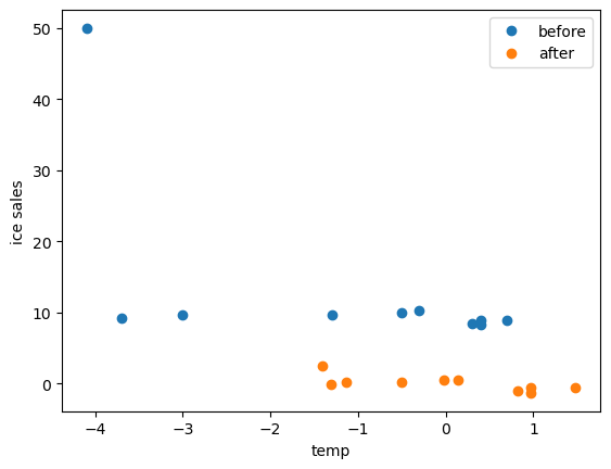
강제로 정규화한 모습이다.
transformr.inverse_transform(transformr.fit_transform(df_train))C:\Users\hollyriver\anaconda3\envs\py\lib\site-packages\sklearn\base.py:464: UserWarning: X does not have valid feature names, but PowerTransformer was fitted with feature names
warnings.warn(array([[-4.1 , 50. ],
[-3.7 , 9.2341745 ],
[-3. , 9.64277825],
[-1.3 , 9.65789368],
[-0.5 , 9.98778744],
[-0.3 , 10.20595116],
[ 0.3 , 8.48692458],
[ 0.4 , 8.81722682],
[ 0.4 , 8.27315516],
[ 0.7 , 8.8637837 ]])df_train| temp | ice_sales | |
|---|---|---|
| 0 | -4.1 | 50.000000 |
| 1 | -3.7 | 9.234175 |
| 2 | -3.0 | 9.642778 |
| 3 | -1.3 | 9.657894 |
| 4 | -0.5 | 9.987787 |
| 5 | -0.3 | 10.205951 |
| 6 | 0.3 | 8.486925 |
| 7 | 0.4 | 8.817227 |
| 8 | 0.4 | 8.273155 |
| 9 | 0.7 | 8.863784 |
어차피 역변환 할 수 있는 것은 상관이 없다.
E. 교호작용의 존재
문제 : 설명 변수 간의 상호작용이 있는 경우, 이를 고려하지 않으면 데이터를 잘 설명하지 못할 수 있음.
- 해결방안
- 교호작용이 있는 열들의 값끼리 곱함
- 교호작용에 영향을 받지 않는 모델 사용 >
sklearn.tree.DecisionTreeRegressor()
- 교호작용이 있는 열을 곱함
df_train = pd.read_csv('https://raw.githubusercontent.com/guebin/MP2023/main/posts/weightloss.csv')
df_train| Supplement | Exercise | Weight_Loss | |
|---|---|---|---|
| 0 | False | False | -0.877103 |
| 1 | True | False | 1.604542 |
| 2 | True | True | 13.824148 |
| 3 | True | True | 13.004505 |
| 4 | True | True | 13.701128 |
| ... | ... | ... | ... |
| 9995 | True | False | 1.558841 |
| 9996 | False | False | -0.217816 |
| 9997 | False | True | 4.072701 |
| 9998 | True | False | -0.253796 |
| 9999 | False | False | -1.399092 |
10000 rows × 3 columns
df_train.pivot_table(index = 'Supplement', columns = 'Exercise', values = 'Weight_Loss', aggfunc = 'mean')| Exercise | False | True |
|---|---|---|
| Supplement | ||
| False | 0.021673 | 4.991314 |
| True | 0.497573 | 14.966363 |
둘 다 했을 때 가장 평균이 높고, 각각 하는 것만으로는 그렇게 큰 영향은 없는 것 같다.
교호작용을 고려하지 않은 분석
## 1
X = df_train.drop('Weight_Loss', axis = 1)
y = df_train.Weight_Loss

## 2
predictr = sklearn.linear_model.LinearRegression()

## 3
predictr.fit(X, y)

## 4
predictr.score(X, y)0.8208414124769222predictr.coef_array([5.21904037, 9.74766346])보충제는 5kg, 운동은 10kg의 감량효과가 있다고 추정하고 있다.
df_train.assign(Weight_Loss_hat = predictr.predict(X)).drop('Weight_Loss', axis = 1)\
.pivot_table(index = 'Supplement', columns = 'Exercise', values = 'Weight_Loss_hat', aggfunc = 'mean')| Exercise | False | True |
|---|---|---|
| Supplement | ||
| False | -2.373106 | 7.374557 |
| True | 2.845934 | 12.593598 |
예측값과 실제 값의 차이가 크다.
교호작용을 고려한 분석
df_train.assign(Interaction = df_train.Supplement * df_train.Exercise)| Supplement | Exercise | Weight_Loss | Interaction | |
|---|---|---|---|---|
| 0 | False | False | -0.877103 | False |
| 1 | True | False | 1.604542 | False |
| 2 | True | True | 13.824148 | True |
| 3 | True | True | 13.004505 | True |
| 4 | True | True | 13.701128 | True |
| ... | ... | ... | ... | ... |
| 9995 | True | False | 1.558841 | False |
| 9996 | False | False | -0.217816 | False |
| 9997 | False | True | 4.072701 | False |
| 9998 | True | False | -0.253796 | False |
| 9999 | False | False | -1.399092 | False |
10000 rows × 4 columns
## 1
_df = df_train.assign(Interaction = df_train.Supplement * df_train.Exercise)
X = _df.drop('Weight_Loss', axis = 1)
y = _df.Weight_Loss

## 2
predictr = sklearn.linear_model.LinearRegression()

## 3
predictr.fit(X, y)

## 4
predictr.score(X, y)0.9727754257714795정확도가 개선되었다.
df_train.assign(Weight_Loss_hat = predictr.predict(X)).drop('Weight_Loss', axis = 1)\
.pivot_table(index = 'Supplement', columns = 'Exercise', values = 'Weight_Loss_hat', aggfunc = 'mean')| Exercise | False | True |
|---|---|---|
| Supplement | ||
| False | 0.021673 | 4.991314 |
| True | 0.497573 | 14.966363 |
평균을 보면(오차를 제거함) 표본과 동일한 것을 볼 수 있다.
3. 교호작용
### A. 아이스크림 타입 별 판매량
- 왠지 익숙한 데이터
np.random.seed(43052)
temp = pd.read_csv('https://raw.githubusercontent.com/guebin/DV2022/master/posts/temp.csv').iloc[:,3].to_numpy()[:100]
temp.sort()
choco = 40 + temp * 2.0 + np.random.randn(100)*3
vanilla = 60 + temp * 5.0 + np.random.randn(100)*3
df1 = pd.DataFrame({'temp':temp,'sales':choco}).assign(type='choco')
df2 = pd.DataFrame({'temp':temp,'sales':vanilla}).assign(type='vanilla')
df_train = pd.concat([df1,df2])
df_train| temp | sales | type | |
|---|---|---|---|
| 0 | -4.1 | 32.950261 | choco |
| 1 | -3.7 | 35.852524 | choco |
| 2 | -3.0 | 37.428335 | choco |
| 3 | -1.3 | 38.323681 | choco |
| 4 | -0.5 | 39.713362 | choco |
| ... | ... | ... | ... |
| 95 | 12.4 | 119.708075 | vanilla |
| 96 | 13.4 | 129.300464 | vanilla |
| 97 | 14.7 | 136.596568 | vanilla |
| 98 | 15.0 | 136.213140 | vanilla |
| 99 | 15.2 | 135.595252 | vanilla |
200 rows × 3 columns
set(df_train.type){'choco', 'vanilla'}plt.plot(df_train.loc[df_train.type == 'choco'].temp, df_train.loc[df_train.type == 'choco'].sales, 'o', label = 'choco')
plt.plot(df_train.loc[df_train.type != 'choco'].temp, df_train.loc[df_train.type != 'choco'].sales, 'o', label = 'vanilla')
plt.legend()
plt.show()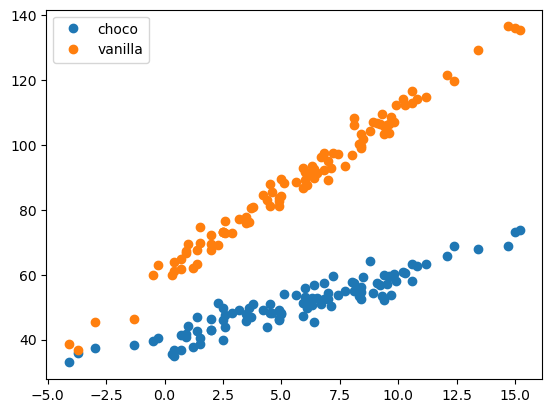
- 아이스크림의 종류에 따라 온도가 판매량에 미치는 정도가 다를 것으로 예상된다.
아이스크림 종류와 온도간에 교호작용이 있다.
교호작용을 고려하지 않은 경우
## 1
X = pd.get_dummies(df_train.drop('sales', axis = 1))
y = df_train.sales

## 2
predictr = sklearn.linear_model.LinearRegression()

## 3
predictr.fit(X, y)

## 4
predictr.score(X, y)0.9249530603100549이것만으로도 나름 높은 점수가 나오긴 했지만… 언제나 개선할 수 있는 건 개선해야 한다.
_df = df_train.assign(sales_hat = predictr.predict(X))plt.plot(df_train.loc[df_train.type == 'choco'].temp, df_train.loc[df_train.type == 'choco'].sales, 'o', label = 'choco')
plt.plot(df_train.loc[df_train.type != 'choco'].temp, df_train.loc[df_train.type != 'choco'].sales, 'o', label = 'vanilla')
plt.plot(df_train.loc[df_train.type == 'choco'].temp, _df.loc[df_train.type == 'choco'].sales_hat, '--', color = 'C0')
plt.plot(df_train.loc[df_train.type != 'choco'].temp, _df.loc[df_train.type != 'choco'].sales_hat, '--', color = 'C1')
plt.legend()
plt.show()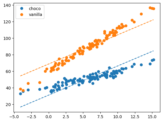
마음속의 언더라잉과 맞지 않는다 : 언더피팅된 상황이다.
교호작용을 고려
van = pd.get_dummies(df_train.type, drop_first = True)*1
van| vanilla | |
|---|---|
| 0 | 0 |
| 1 | 0 |
| 2 | 0 |
| 3 | 0 |
| 4 | 0 |
| ... | ... |
| 95 | 1 |
| 96 | 1 |
| 97 | 1 |
| 98 | 1 |
| 99 | 1 |
200 rows × 1 columns
_df = df_train.assign(Interaction = df_train.temp * van.vanilla)
_df| temp | sales | type | Interaction | |
|---|---|---|---|---|
| 0 | -4.1 | 32.950261 | choco | -0.0 |
| 1 | -3.7 | 35.852524 | choco | -0.0 |
| 2 | -3.0 | 37.428335 | choco | -0.0 |
| 3 | -1.3 | 38.323681 | choco | -0.0 |
| 4 | -0.5 | 39.713362 | choco | -0.0 |
| ... | ... | ... | ... | ... |
| 95 | 12.4 | 119.708075 | vanilla | 12.4 |
| 96 | 13.4 | 129.300464 | vanilla | 13.4 |
| 97 | 14.7 | 136.596568 | vanilla | 14.7 |
| 98 | 15.0 | 136.213140 | vanilla | 15.0 |
| 99 | 15.2 | 135.595252 | vanilla | 15.2 |
200 rows × 4 columns
## 1
X = pd.get_dummies(_df.drop('sales', axis = 1), drop_first = True)
y = _df.sales

## 2
predictr = sklearn.linear_model.LinearRegression()

## 3
predictr.fit(X, y)

## 4
predictr.score(X, y)0.9865793819066231점수가 훨씬 높게 나왔다.
__df = _df.assign(sales_hat = predictr.predict(X))
__df| temp | sales | type | Interaction | sales_hat | |
|---|---|---|---|---|---|
| 0 | -4.1 | 32.950261 | choco | -0.0 | 31.403121 |
| 1 | -3.7 | 35.852524 | choco | -0.0 | 32.209366 |
| 2 | -3.0 | 37.428335 | choco | -0.0 | 33.620295 |
| 3 | -1.3 | 38.323681 | choco | -0.0 | 37.046835 |
| 4 | -0.5 | 39.713362 | choco | -0.0 | 38.659325 |
| ... | ... | ... | ... | ... | ... |
| 95 | 12.4 | 119.708075 | vanilla | 12.4 | 122.492017 |
| 96 | 13.4 | 129.300464 | vanilla | 13.4 | 127.521196 |
| 97 | 14.7 | 136.596568 | vanilla | 14.7 | 134.059129 |
| 98 | 15.0 | 136.213140 | vanilla | 15.0 | 135.567883 |
| 99 | 15.2 | 135.595252 | vanilla | 15.2 | 136.573719 |
200 rows × 5 columns
plt.plot(df_train.loc[df_train.type == 'choco'].temp, df_train.loc[df_train.type == 'choco'].sales, 'o', label = 'choco')
plt.plot(df_train.loc[df_train.type != 'choco'].temp, df_train.loc[df_train.type != 'choco'].sales, 'o', label = 'vanilla')

plt.plot(df_train.loc[df_train.type == 'choco'].temp, __df.loc[df_train.type == 'choco'].sales_hat, '--', color = 'C0')
plt.plot(df_train.loc[df_train.type != 'choco'].temp, __df.loc[df_train.type != 'choco'].sales_hat, '--', color = 'C1')

plt.legend()
plt.show()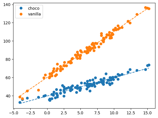
predictr.coef_array([ 2.01561216, 3.01356716, 20.46306209])모델이 언더라잉을 잘 따라가는 것을 볼 수 있다.(애초에 계수가 세개가 됨…)
B. 교호작용, tree
sklearn.tree.DecisionTreeRegressor()를 사용하면 교호작용을 손쉽게 적합할 수 있다.
np.random.seed(43052)
temp = pd.read_csv('https://raw.githubusercontent.com/guebin/DV2022/master/posts/temp.csv').iloc[:,3].to_numpy()[:100]
temp.sort()
choco = 40 + temp * 2.0 + np.random.randn(100)*3
vanilla = 60 + temp * 5.0 + np.random.randn(100)*3
df1 = pd.DataFrame({'temp':temp,'sales':choco}).assign(type='choco')
df2 = pd.DataFrame({'temp':temp,'sales':vanilla}).assign(type='vanilla')
df_train = pd.concat([df1,df2])
df_train| temp | sales | type | |
|---|---|---|---|
| 0 | -4.1 | 32.950261 | choco |
| 1 | -3.7 | 35.852524 | choco |
| 2 | -3.0 | 37.428335 | choco |
| 3 | -1.3 | 38.323681 | choco |
| 4 | -0.5 | 39.713362 | choco |
| ... | ... | ... | ... |
| 95 | 12.4 | 119.708075 | vanilla |
| 96 | 13.4 | 129.300464 | vanilla |
| 97 | 14.7 | 136.596568 | vanilla |
| 98 | 15.0 | 136.213140 | vanilla |
| 99 | 15.2 | 135.595252 | vanilla |
200 rows × 3 columns
아까와 동일한 자료를 tree로 분석해보자…
## 1
X = pd.get_dummies(df_train.drop('sales', axis = 1), drop_first = True)
y = df_train.sales

## 2
predictr = sklearn.tree.DecisionTreeRegressor()

## 3
predictr.fit(X, y)

## 4
predictr.score(X, y)0.9963887702553287높은 스코어가 나온다.(오버피팅된 것은 아닐까?)
_df = df_train.assign(sales_hat = predictr.predict(X))
_df| temp | sales | type | sales_hat | |
|---|---|---|---|---|
| 0 | -4.1 | 32.950261 | choco | 32.950261 |
| 1 | -3.7 | 35.852524 | choco | 35.852524 |
| 2 | -3.0 | 37.428335 | choco | 37.428335 |
| 3 | -1.3 | 38.323681 | choco | 38.323681 |
| 4 | -0.5 | 39.713362 | choco | 39.713362 |
| ... | ... | ... | ... | ... |
| 95 | 12.4 | 119.708075 | vanilla | 119.708075 |
| 96 | 13.4 | 129.300464 | vanilla | 129.300464 |
| 97 | 14.7 | 136.596568 | vanilla | 136.596568 |
| 98 | 15.0 | 136.213140 | vanilla | 136.213140 |
| 99 | 15.2 | 135.595252 | vanilla | 135.595252 |
200 rows × 4 columns
plt.plot(df_train.loc[df_train.type == 'choco'].temp, df_train.loc[df_train.type == 'choco'].sales, 'o', label = 'choco', alpha = 0.5)
plt.plot(df_train.loc[df_train.type != 'choco'].temp, df_train.loc[df_train.type != 'choco'].sales, 'o', label = 'vanilla', alpha = 0.5)

plt.plot(df_train.loc[df_train.type == 'choco'].temp, _df.loc[df_train.type == 'choco'].sales_hat, '--', color = 'C0')
plt.plot(df_train.loc[df_train.type != 'choco'].temp, _df.loc[df_train.type != 'choco'].sales_hat, '--', color = 'C1')

plt.legend()
plt.show()
오차항까지 적합하고는 있으나… 처음 교호작용을 고려하지 않은 모델보다 성능은 좋은 것 같다. 따라서 이는 상당히 유용하다.